If you’re looking for the math behind the model and full run-down of how oxygen deficiency hazards are evaluated at LBNL, then you’ve come to the right place. If you just want an overview of the process and the requirements, check out the page on Oxygen Deficiency Hazards and Asphyxiation.
Fermilab essentially wrote the book (or at least the chapter) on oxygen deficiency hazard (ODH) risk assessment. As the nation’s preeminent particle physics and accelerator laboratory, Fermilab utilizes massive volumes of cryogenic liquids in some very unique situations, leading to some very unique oxygen deficiency hazard scenarios. Here at LBNL, we base all of our own oxygen deficiency hazard assessments on Fermilab’s model and methods, and we have adapted a simplified process as an initial screening tool for low-risk applications. Here you’ll find an abbreviated explanation of Fermilab’s model, as well as the details of how we have adapted the model to suit our own needs at LBNL.
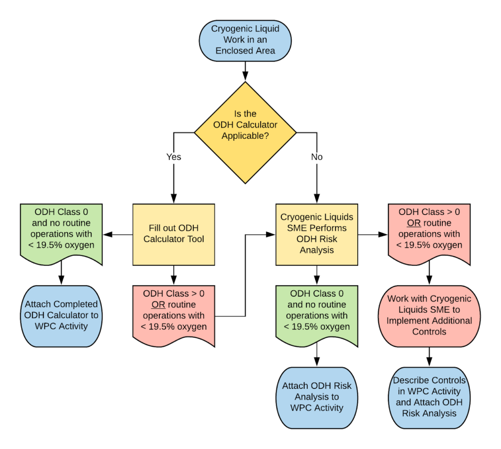
ODH Analysis Process Overview
Oxygen Deficiency Modeling Details
There are two main pieces to determining the oxygen deficiency hazard (ODH) class of a given room:
- a model for determining the oxygen concentration in a given room based on the volume of inert gas released and the ventilation provided to the room
- a risk analysis to estimate the fatality rate for the given release scenario based on the risk of death from oxygen deficiency and the probability of the event occurring
Both parts have their drawbacks and limitations, but the overall process is designed to be done by a single subject matter expert in a matter of a few hours to several days depending on the complexity of the system, and to provide a conservative estimate of the risk to the worker. The subject matter expert is expected to use professional judgement to determine if and how the model needs to be modified. For example, the subject matter expert may measure the ventilation rate of a room and visualize the air movement with a smoke generator, and decide that there is insufficient air mixing to justify the assumption that the entire room volume is perfectly mixed. In such a case, the subject matter expert may reduce the effective volume of the area. The risk analysis portion is fairly straightforward. For any scenario that results in an oxygen deficient atmosphere, we use a formula to estimate the probability of a fatality for someone exposed to that scenario. We have adopted the Fermilab model, which assumes a logarithmic relationship between the probability of a fatality and the lowest expected oxygen concentration, with limits set at p=0 at 135mmHg oxygen partial pressure and above (18% by volume at 760mmHg or 101kPa of pressure) and p=1 (or 100%) at 65mmHg oxygen partial pressure and below (8.8% oxygen by volume at 760mmHg or 101kPa of pressure). This yields the formula, f = 10((65-PO2)/10), where f is in fatalities per occurrence. Of course the formula may not accurately represent the risk of death for all persons, but is based on what data is available. The original equation uses units of mmHg, but we can convert to kiloPascals to obtain: f = 10((8.67-PO2)/10). Along with the probability of a fatality if that scenario occurs, we determine the probability that such a scenario will actually occur (P, expressed per hour). For any routine operation, we assign a value of 1, or 100% probability of occurrence. For failure scenarios, we rely on operating experience of how often certain parts fail and in what ways. Given that we are in California and situated very near a fault line, we also include an earthquake scenario, in which we assume that all cryogenic liquid storage containers will fail completely and release into the room. The probability of an earthquake is based on the USGS earthquake forecast, which predicts how likely any region is to experience a magnitude 6.7+ earthquake in the next 30 years. The most recent prediction is 72% for the SF Bay Area (in the next 30 years). So from there, we back-calculate from 0.72 per 30 years to 4.84×10⁻⁶ per hour (see below for derivation). Once all of the possible scenarios have been assigned a fatality rate and a probability, these can be summed to give an overall fatality rate for a person occupying the room, expressed as fatalities per hour, φ = ΣFiPi, which is always ≤ 1. Clearly, a value anywhere near 1 is unacceptable. Below that, we assign a hazard class rating based on the following cutoffs:
| Fatality Rate (φ, per hour) | ODH Class | Explanation |
|---|---|---|
| φ < 10-7 | 0 | less than 1 fatality in 10 million hours |
| 10-7 ≤ φ < 10-5 | 1 | less than 1 fatality in 100,000 hours |
| 10-5 ≤ φ < 10-3 | 2 | less than 1 fatality in 1,000 hours |
Routine Operations and Failure Analysis
Modeling the Expected Equilibrium Oxygen Concentration
To calculate the probability of a fatality we need to know the oxygen concentration in the room that will result from each scenario. This model is a little more complicated because we need to factor in the effect of the ventilation system constantly removing air from the room and/or supplying some volume of fresh air. The conceptual basis of the model has a number of assumptions built in. The first, and arguably most problematic, assumption is that the inert gas will perfectly and instantaneously mix with the air in the room. As a corollary, we assume that the ventilation system removes air from the room with the same oxygen concentration as that within the room overall. And we assume that the ventilation supplies air with an oxygen concentration of 20.9% by volume, although the model can be adapted for some portion of air recirculation.
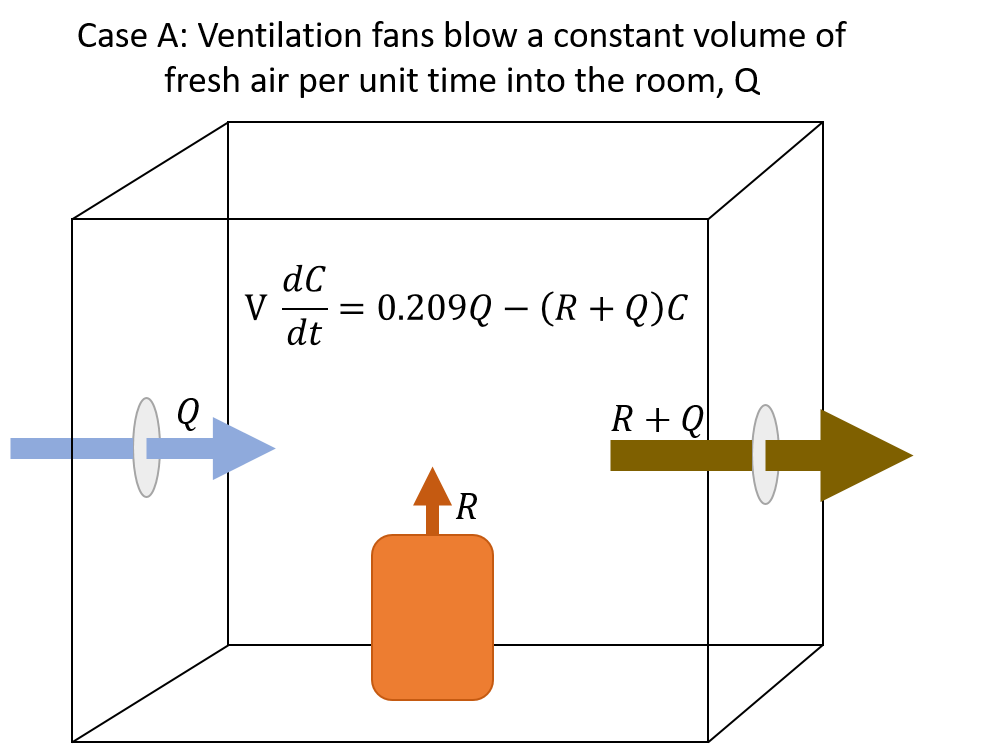
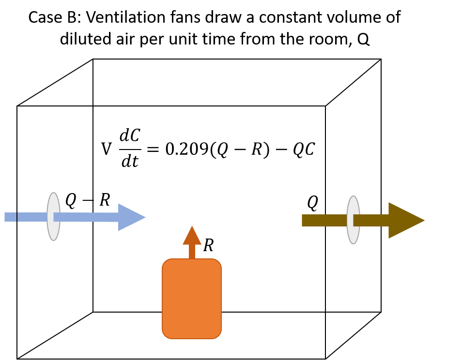
The model takes a room with some internal volume, V. There is a source of inert gas that produces some volume of inert gas per unit of time, R, and a ventilation system that moves some constant volume of gas either into or out of the room per unit time, Q. The model diverges here based on whether the ventilation system is blowing fresh air into the room (case A) or drawing the inert gas/air mixture from the room (cases B and C, depending on whether the ventilation rate exceeds the rate of inert gas production).
The illustrations to the right give a visual overview of each case, and display the differential equation for the mass balance of oxygen.
Nearly every laboratory space at LBNL utilizes ventilation systems that maintain a constant draw from the room, with make-up air provided on demand, to keep the room under slight negative pressure with respect to non-laboratory spaces such as offices and hallways. It is also very rare that the “spill rate” of inert gas into the room exceeds the ventilation rate. Therefore we almost exclusively use Case B.
The model returns a value in percent oxygen by volume. This value must be converted to a partial pressure of oxygen based on the absolute atmospheric pressure. Because LBNL is located at an elevation of approximately 1,000 feet above sea level, we use a value of 730mmHg for atmospheric pressure, rather than the standard 760mmHg assumed at sea level.

Modeling the Spill Rate, R
To obtain a spill rate, we can often use known or estimated rates from manufacturer information from a piece of equipment, or from the operational experience of people who work with the system. Safety factors are generally applied to the spill rate to allow for error from such factors as degradation of insulation or operational variability. One example of this is using the manufacturer-provided “loss rate” of a Dewar, which is usually expressed in liters of cryogenic liquid per day. This is converted to liters of gas per hour. Another example is a cryostat that must be topped off with 4L of liquid nitrogen each day of operation. It can be assumed then that 4L of liquid nitrogen are released into the room per 24 hours, and this is again converted to liters of gas per hour.
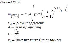
Sometimes it is necessary to calculate a spill rate, especially for failure scenarios. Leaks from plumbing failures or hose disconnections are the most common failure scenarios. In this case, a simple fluid model for choked flow is employed to estimate the release rate based on the size of the opening, the fluid properties, and the pressure upstream of the leak. In rare cases, an unchoked flow model may be used instead, based on the pressure and size of the opening.
Examples
Example ODH: Argon flow through a purification column and into a Dewar
In this situation, liquid argon from a pressurized Dewar is flowed through a purification column and into a non-pressurized Dewar. To determine the release of argon into the room a heat exchange model was employed, assuming that the purification column and non-pressurized Dewar started at room temperature and would be cooled to liquid argon temperature. Multiple safety factors were applied. The following visualization includes a one-time cool-down of the purifier and Dewar, plus an ongoing release rate from the purification process.

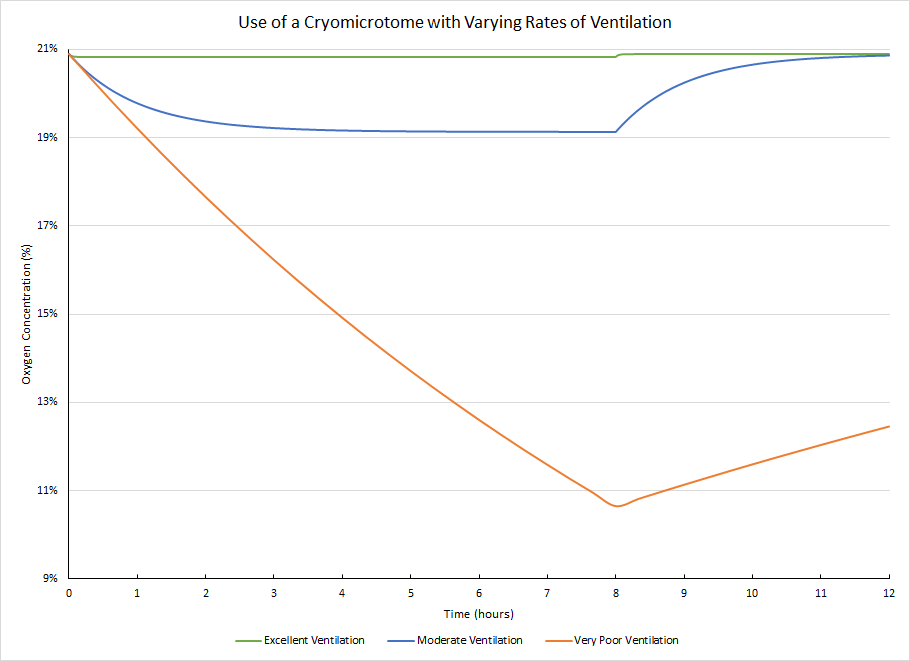
Example ODH: Operation of a Cryomicrotome
In this situation, a cryomicrotome is set up in a small room. During normal operation, the manufacturer states that the instrument will use less than 10L of liquid nitrogen over an 8 hour work shift. A safety factor of 2 was applied, to give a release rate of 2.5L liquid nitrogen per hour, or 1,740L nitrogen gas per hour. Here you can see the difference between scenarios where the microtome is run continuously for an 8 hour work shift with different rates of ventilation. The actual ventilation in the room was measured and is the example used here for “excellent ventilation”.
Derivation of an Earthquake Rate per Hour
The following derivation is the best that the cryo SME has at this point. If there is a flaw in the logic behind it, or if you have a better method, please let me know! Huge thanks to Dr. Fisher at Lawrence Livermore National Laboratory for help with this work.
We start with the probability of at least one earthquake of magnitude 6.7+ occurring in the next 30 years, denoted P(Et) = 0.72. This number is based on the USGS UCERF3 Earthquake Forecast for the San Francisco Area, which includes events on the Hayward, Calaveras, and Northern San Andreas faults.
This means that there is a probability that we will have no earthquakes of magnitude 6.7+ in the next 30 years, denoted P(E’t), of 0.28.
From here, we wish to determine the probability of an earthquake occurring in some fraction of that time, t/α, denoted as P(Et/α). To do this, we work backward from the probability of an earthquake not occurring in time t/α, denoted P(E’t/α), because in order for there not to be an earthquake in the next 30 years, there must not be an earthquake in each and every fraction of that time.
We know that the probability of A and B is P(A)P(B). So the probability of there being no earthquake in each and every time fraction, t/α, is P(E’t) = P(E’t/α)α. Rearranging to solve for P(E’t/α) we see that P(E’t/α) = P(E’t)1/α.
And since we know that P(Et/α) + P(E’t/α) = 1, we know that P(Et/α) = 1 – P(E’t/α) = 1 – P(E’t)(1/α).
There are 262,800 hours in 30 years. Therefore P(Et/α) = 1 – 0.28(1/262,800) = 4.84×10⁻⁶.
When compared to a more rudimentary method of determining the probability of an earthquake per hour, where the probability per 30 years is simply divided by the number of hours in 30 years (resulting in a rate of 2.74×10⁻⁶), this method provides a higher earthquake rate and is thus a more conservative estimation of our earthquake rate.

